Quick start

Install EpiAware and build your first models — composing distributions and assembling a joint model you can fit.

EpiAware is a set of small Julia packages that compose into infectious disease models. This shows the two ways you work with them: compose the distributions your data need, and assemble a whole model you can fit. The figures below are produced by running the code in CI, so they track the current packages.

New to Julia? Start with the Using Julia guide.

Install

Most packages are early and installed from GitHub:

using Pkg
Pkg.add(url = "https://github.com/EpiAware/ComposedDistributions.jl")
Pkg.add(url = "https://github.com/EpiAware/ComposableTuringIDModels.jl")

Compose a delay chain

A case moves through events — infection, symptom onset, hospital admission, death — each a delay on the one before. Chain them with Sequential, and the tree prints its own structure:

using ComposedDistributions, Distributions

chain = Sequential([
    Gamma(2.0, 1.5),      # infection → onset
    LogNormal(1.0, 0.5),  # onset → admission
    Gamma(2.0, 3.0),      # admission → death
])

Sequential (3 steps)
├─ step_1: Gamma{Float64}(α=2.0, θ=1.5)
├─ step_2: LogNormal{Float64}(μ=1.0, σ=0.5)
└─ step_3: Gamma{Float64}(α=2.0, θ=3.0)

The delay from infection to each event is the convolution of the steps so far — convolved composes them, and the result is an ordinary distribution you can pdf, rand, and plot:

using CairoMakie

to_onset     = Gamma(2.0, 1.5)
to_admission = convolved(to_onset, LogNormal(1.0, 0.5))
to_death     = convolved(to_admission, Gamma(2.0, 3.0))

ts = 0:0.1:32
fig = Figure()
ax = Axis(fig[1, 1]; xlabel = "days since infection", ylabel = "density")
for (d, label) in [(to_onset, "onset"), (to_admission, "admission"),
                   (to_death, "death")]
    lines!(ax, ts, pdf.(d, ts); label, linewidth = 3)
end
axislegend(ax)
fig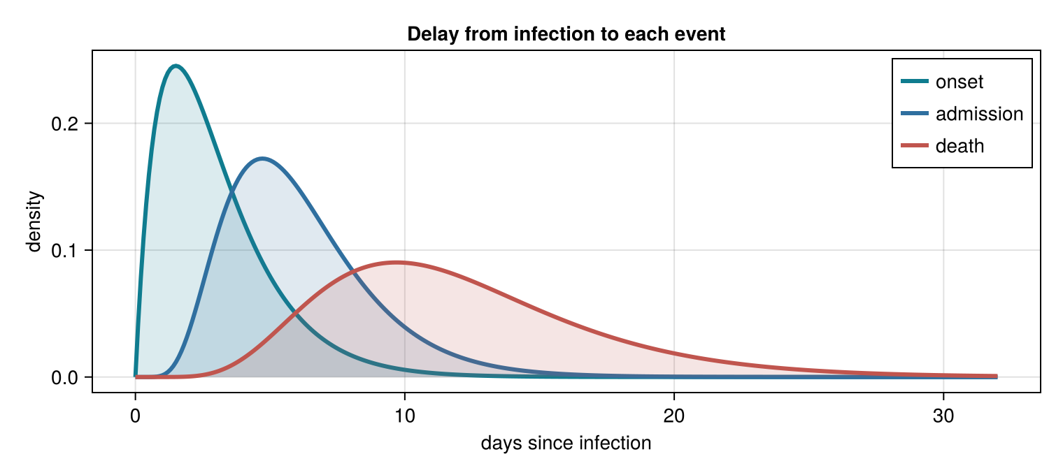

Density of the delay from infection to onset, admission, and death

Build and simulate a model

Assemble a model from interchangeable parts — a latent random walk driving direct infections, observed with Poisson error — with IDModel, which also prints its structure:

using ComposableTuringIDModels, Distributions

model = IDModel(
    DirectInfections(; Z = RandomWalk(), initialisation_prior = Normal()),
    PoissonError())

IDModel
├─ infection: DirectInfections
│  └─ Z: RandomWalk
│     └─ ϵ_t: HierarchicalNormal
└─ observation: PoissonError

as_turing_model turns the assembly into a Turing model. Pass missing for the data and it simulates from the prior — here 30 draws of a 40-day outbreak:

n = 40
simulator = as_turing_model(model, missing, n)
sims = [simulator() for _ in 1:30]   # each has generated_y_t, I_t, Z_t

fig = Figure()
ax = Axis(fig[1, 1]; xlabel = "day", ylabel = "cases")
for s in sims
    lines!(ax, 1:n, s.generated_y_t; color = (:steelblue, 0.28))
end
fig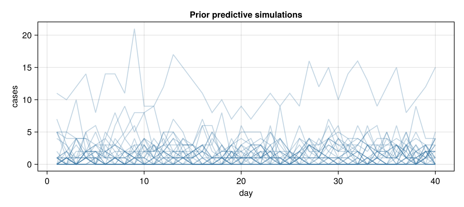

Thirty prior predictive case trajectories over 40 days

To fit real data, pass the case series instead of missing and sample:

turing_model = as_turing_model(model, cases, length(cases))
# 1000 draws across 2 chains, one per core
chain = sample(turing_model, NUTS(), MCMCThreads(), 1_000, 2)

Browse the packages and open each one’s documentation.
Each package’s docs include worked examples that go further.
Ready to contribute or bring a use case? Get involved.

Install

Compose a delay chain

Build and simulate a model

Next